Subsection7.3.1Definition and Basic Properties of Vector Fields and Differential One-Forms
We start with an initial definition of a vector field in a Euclidean domain; it is to be modified later to be suitable in a more general context such as on a differentiable surface.
Definition7.3.1.Vector Field in a Euclidean Domain.
Let \(U\subset \bbR^{n}\) be open. A vector field in \(U\) is an \(\bbR^{n}\)-valued function \(X:\bx\in U\mapsto \bbR^{n}\text{.}\) A vector field \(X(\bx)\) is continuous (differentiable) in \(U\) if \(X(\bx)\) as an \(\bbR^{n}\)-valued function is continuous (differentiable) in \(U\text{.}\)
We will use a vector field mostly in the operation of taking directional derivatives of differentiable functions. First, recall the directional derivative of a differentiable function \(f\) in \(\bbR^{n}\) in the direction \({\mathbf v}\) at a point \(P\text{:}\)
where \({\mathbf v}=(v^{1},\ldots, v^{n})\text{.}\) This relation holds for any differentiable curve \(\vec{\gamma}(t)\) passing through \(P\) at \(t=0\) and \(\vec{\gamma}'(0)={\mathbf v}\text{:}\)
\({\mathbf v}\) is called a tangent vector at \(P\text{.}\) The set of tangent vectors at \(P\) forms a vector space, called the tangent space of \({\mathbb R}^{n}\) at \(P\text{,}\) and is denoted as \({\mathbb R}^{n}_{P}\text{.}\) For the situation here, \({\mathbb R}^{n}_{P}\) is simply a copy of \(\bbR^{n}\text{,}\) and \({\mathbb R}^{n}_{P}\) at different \(P\) are identified with each other in a natural way. But we will see that this is not the case when we discuss the tangent space of a differentiable surface, as there is no obvious natural relations between vectors at different points, and it is important to associate a tangent vector to a specific point.
Suppose that \(X(\bx)\) is a continuous vector field on \(U\) and \(f(\bx)\) is a continuously differentiable function on \(U\text{,}\) then at each \(\bx\in U\text{,}\)\(X(\bx)\) is a tangent vector at \(\bbR^{n}_{\bx}\) and \(D_{X(\bx)}f(\bx)\) is a continuous function on \(U\text{.}\)
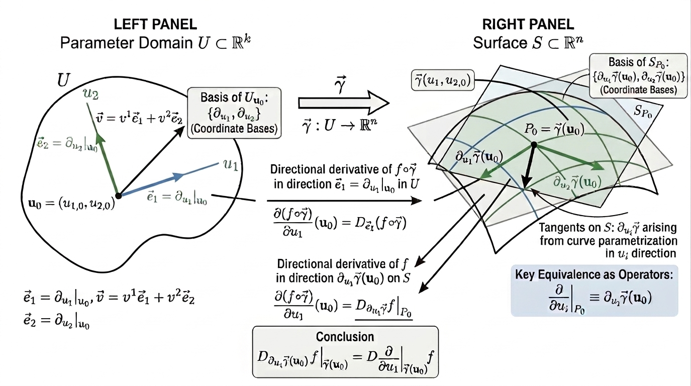
The discussions in the previous paragraphs generalize to a (differentiable) surface in \({\mathbb R}^{n}\text{.}\) We will first work with a patch of a differentiable surface as given by a differentiable map \(\vg (\bu): U\mapsto {\mathbb R}^{n}\) defined for the parameter \(\bu\in U \subset \bbR^{k}\) for some open domain \(U\text{.}\) A differentiable curve on the surface through \(P_{0}=\vg(\bu_{0})\) is given in terms of \(\vg(\bu(t))\text{,}\) where \(\bu(t)\) is a differentiable curve in the parameter domain \(U\) with \(\bu(0)=\bu_{0}\text{.}\) Then the chain rule
\begin{equation*}
\left[ \vg(\bu(t)) \right]' =[D_{\bu}\vg(\bu(t))] \bu'(t)=\sum_{i=1}^{k} \frac{du_{i}}{dt} \partial_{u_{i}}\vg(\bu(t))
\text{ for } t \text{ near } 0
\end{equation*}
implies that the tangent of the curve \(\vg(\bu(t))\) at \(P_{0}\text{,}\)\(\left[ \vg(\bu(t)) \right]'|_{t=0}\text{,}\) is a linear combination of \(\partial_{u_{i}}\vg(\bu_0)\text{,}\) where \(\partial_{u_{i}}\vg(\bu_0)\) is an alternative notation for \(D_{\be_{i}}\vg(\bu_0)\text{,}\) namely, the partial derivative of \(\vg(\bu)\) with respect to its \(i\)th coordinate. Note that every such tangent vector lies in the span of these \(k\) vectors, which forms the tangent space of the surface at \(P_{0}\text{.}\)
In order for such a parametrization \(\vg(\bu)\) to represent a geometric \(k\)-dimensional surface, we require that these \(k\) vectors be linearly independent so the tangent space to the surface is \(k\)-dimensional, namely the matrix \([\partial_{u_{1}}\vg(\bu_0)\, \ldots\, \partial_{u_{k}}\vg(\bu_0)]\) has rank \(k\text{.}\) Let \(S\) denote this patch of differentiable surface. Then there is a well defined tangent space \(S_{\vg(\bu)}\) for every \(\bu\) (or rather for every point \(\vg(\bu)\) on \(S\)). When \(\vg(\bu)\) is continuously differentiable, we have a sense that the tangent space \(S_{\vg(\bu)}\) varies continuously with \(\bu\text{.}\) But that is not a topic to be taken up now. Instead, we first focus on how a tangent vector is used to compute the directional derivative of a differentiable function.
If \(f\) is a differentiable function defined on \(\bbR^{n}\text{,}\) then its restriction to the surface \(S\) becomes a function on the surface. To consider its differentiability properties on the surface, we use the parametrization \(\vg(\bu)\) to get a function \(f\circ \vg\) in the parameter domain of \(\bu\text{,}\) then the directional derivative of \(f\) at \(P_{0}\) in the direction of \(\partial_{u_i}\vg(\bu_0)\) is given by
It is this kind of consideration that makes it natural to use \(\frac{\partial }{\partial u_{i}}\Big|_{\vg(\bu_0)}\) to represent the tangent vector \(\partial_{u_i}\vg(\bu_0)\) to the surface at \(P_{0}=\vg(\bu_0)\text{,}\) when \(\vg(\bu)\) is a parametric representation of the surface. Namely,
\(\frac{\partial \vg}{\partial u_{i}}=\partial_{u_i}\vg\) is a geometric tangent vector to the surface \(\bx=\vg(\bu)\) at \(\vg(\bu)\) arising from a curve whose parametrization in the \(\bu\) parameter space runs along the \(u_{i}\) direction.
\(\frac{\partial (f\circ \vg)}{\partial u_{i}}=D_{\partial_{u_i}\vg}f\) means that, as an operator, \(\frac{\partial }{\partial u_{i}}\) represents directional derivative in the direction of the tangent \(\partial_{u_i}\vg\text{.}\)
\begin{equation*}
D_{\partial_{u_i}\vg(\bu_0)} f \Big|_{\vg(\bu_0)}=D_{\frac{\partial }{\partial u_{i}}\Big|_{\vg(\bu_0)}}f .
\end{equation*}
In this notation, \(\left\{ \frac{\partial }{\partial u_{1}}\Big|_P, \ldots, \frac{\partial }{\partial u_{k}}\Big|_P\right\}\) forms a basis of \(S_{P}\text{.}\) The advantage of this notation will become clear when a change of variable is used, which would cause a change of basis for the tangent space. We can write any \(\bv\in S_{P}\) as \(\bv=\sum_{i=1}^{k}v^{i}\frac{\partial }{\partial u_{i}}\Big|_P\text{,}\) then
Figure7.3.2.An illustration of tangents on a surface in relation to partial differentiation with respect to the parameter variables generated with the help of Gemini
Definition7.3.3.Vector Field on a Differentiable Surface.
A vector field \(X\) on a differentiable surface \(S\) is a map \(P\in S\mapsto X(P)\in S_{P}\text{.}\) Namely, it assigns to each \(P\in S\) a tangent vector \(X(P)\) to \(S\) at \(P\text{.}\)
When \(S\) is given by a differentiable parametrization \(\vg :U\subset \bbR^{k}\mapsto S\text{,}\) any vector field \(X\) on \(S\) can be represented as \(X(\vg(\bu))=\sum_{i=1}^{k} X_{i}(\bu) \frac{\partial }{\partial u_{i}}\Big|_{\vg(\bu)}.\)\(X\) is said to be a continuous (or continuously differentiable) vector field on \(S\) if the coefficient functions \(X_{i}(\bu)\) are continuous (or continuously differentiable) functions of \(\bu \in U\text{.}\)
We will often write \(\frac{\partial }{\partial u_{i}}\) for \(\frac{\partial }{\partial u_{i}}\Big|_{\vg(\bu)}\) to simplify notations. Note that \(\frac{\partial }{\partial u_{i}}\) is a vector field on \(S\text{,}\) but if the \(u_{i}\)’s are not used in connection with the parametrization, then \(\frac{\partial }{\partial u_{i}}\) also represents a vector field in \(U\text{,}\) which takes the vector \(\be_{i}\) everywhere in \(U\text{.}\) One should watch out for the context in which this notation is used. In the latter context, a vector field in \(U\) is simply an \(R^{k}\)-valued function, so one can take its derivative and in this case \(D_{\bv}\left(\frac{\partial }{\partial u_{i}}\right)=0\) for any \(\bv\in \bbR^{k}_{\bu}\text{,}\) as \(\frac{\partial }{\partial u_{i}}=\be_{i}\) in this context. But in the former context, \(\bv\) should be regarded as the tangent vector \(\frac{d \vg(\bu+t\bv)}{dt}\Big|_{t=0}=D_{\bu}\vg(\bu)=[D\vg(\bu)]\bv \in S_{\vg(\bu)}\) on \(S\text{,}\) and \(D_{\bv}\left(\frac{\partial }{\partial u_{i}}\right)\) should be related to \(D_{[D\vg(\bu)]\bv}\left(\frac{\partial \vg(\bu)}{\partial u_{i}}\right)=\sum_{j=1}^{k}v_j \frac{\partial^2 \vg_(\bu)}{\partial u_j \partial u_{i}}\text{.}\) But this output in \(\bbR^{n}\) may not be a tangent vector to \(S\) at \(\vg(\bu)\text{.}\) There is a way to obtain a tangent vector to \(S\) at \(\vg(\bu)\) through orthogonal projection. This will introduce the notion of covariant differentiation of vector field on \(S\text{.}\) But we will not pursue that topic in this course.
A graph \(G\) of a differentiable function \(h(\bu)\) for \(\bu \in \bbR^{n-1}\) can be parametrized as \(\vg (\bu)=(\bu, h(\bu))\text{.}\) Then the vector field \(\frac{\partial }{\partial u_{i}}\) is simply a coordinate representation for the geometric vector field \((\mathbf e_{i}, \frac{\partial h(\bu) }{\partial u_{i}})\) on \(G\text{,}\) and
\(\{\frac{\partial }{\partial u_{1}}, \ldots, \frac{\partial }{\partial u_{n-1}}\}\) is a basis of \(G_{(\bu, h(\bu))}\text{.}\) In this notation \((1, 0, \cdots, 0)\) is a coordinate representation in this basis for the vector field \(\frac{\partial }{\partial u_{1}}\) for \((\bu, h(\bu))\in G\text{,}\) yet its values at different \(\bu\) (or rather \((\bu, h(\bu))\)) may not be identified as equal to each other. As a consequence, we may not have \(D_{\bv}(\frac{\partial }{\partial u_{1}})=\mathbf 0\) in contrast to the case if \(\{\frac{\partial }{\partial u_{i}}=\be_{i}\}\) is used to represent a basis of the tangent space at a point in the flat Euclidean space.
defines a linear function on \({\mathbb R}^{n}_{P}\text{,}\) thus defines a cotangent vector in \({{\mathbb R}^{n}_{P}}^{*}\text{,}\) called the differential of \(f\) at \(P\text{,}\) and is denoted as \(df(P)\text{.}\) Thus
\begin{equation*}
df(P)({\mathbf v})=D_{{\mathbf v}}f(P) \quad \text{ for all $\bv \in {\mathbb R}^{n}_{P}$.}
\end{equation*}
This definition requires \(f\) to be differentiable in a neighborhood of a point, it naturally defines a field of cotangent vectors in \({{\mathbb R}^{n}_{P}}^{*}\) as \(P\) varies in this neighborhood. It is an example of a one form, and in this case, is called the differential of \(f\text{.}\)
In older texts the differential \(df\) was often used interchangeably with \(\sum_{i=1}^{n}\frac{\partial f}{\partial x_{i}} \Delta x_{i}\) and referred to as the linear approximation to \(f\) at \(P\text{.}\) In the modern treatment, the differential \(df\) is a linear function on tangent vectors, so after taking a tangent vector \(\mathbf v\) as input it gives the linear approximation \(df(P)({\mathbf v})=\sum_{i=1}^{n}\frac{\partial f}{\partial x_{i}} dx_{i}({\mathbf v})
=\sum_{i=1}^{n}v_{i} \frac{\partial f}{\partial x_{i}}\) to the increment of \(f\) at \(P\) along \(\mathbf v\text{.}\)
Note that \(\left\{ dx_{1}\Big|_P, \ldots, dx_{n}\Big|_P\right\}\) forms the dual basis of \(\left\{ \frac{\partial }{\partial x_{1}}\Big|_P, \ldots, \frac{\partial }{\partial x_{n}}\Big|_P\right\}\text{,}\) as
\begin{equation}
dx_{i}(\frac{\partial }{\partial x_{j}})=D_{\frac{\partial }{\partial x_{j}}}x_{i}=\delta_{ij} \text{ for } 1\le i, j \le n.\tag{7.3.2}
\end{equation}
A general one-form can be expressed as \(\sum_{i=1}^{n}\xi_{i}(\bx) dx_{i}\) for some scalar functions \(\xi_{i}(\bx)\text{.}\) It is called continuous (differentiable) if these functions are continuous (differentiable). We will learn later that for a general domain not all continuous one-forms can be the differential \(df\) of some continuously differentiable functions \(f\text{.}\)
The above discussion adapts easily to the context of a differentiable surface such as \(S\) represented in terms of a parametric representation \(\vg (\bu)\) for \(\bu \in U\subset \bbR^{k}\text{.}\) Then \(\left\{ du_{1}\Big|_P, \ldots, du_{k}\Big|_P\right\}\) forms the dual basis of \(\left\{ \frac{\partial }{\partial u_{1}}\Big|_P, \ldots, \frac{\partial }{\partial u_{k}}\Big|_P\right\}\text{.}\) We will use \(du_{i}\) for \(du_{i}\Big|_P\text{.}\) Any one-form on \(S\) can be represented as \(\sum_{i=1}^{k} \alpha_{i}(\bu) du_{i}\) for some functions \(\alpha_{i}(\bu)\text{.}\)
We next study the transformation laws of a vector field and a one-form under a change of coordinates. Suppose that \(\vg^{\dagger}(\bv)\) for \(\bv=( v_{1}, \cdots, v_{k})\in V\subset \bbR^{k}\) provides another parametrization for the same \(S\) via the relation \(\bv=F(\bu)\) for some continuously differentiable \(F\) with continuously differentiable inverse: \(\vg^{\dagger}(F(\bu))= \vg(\bu)\text{.}\) A parametrization with this property is called admissible.
\((f\circ \vg)(\bu)\) and \((f\circ \vg^{\dagger})(\bv)\) are simply two different coordinate representations of the same function \(f\text{,}\) so we have the following
This is the transformation law between the two bases \(\left\{ \frac{\partial }{\partial u_{1}}\Big|_P, \ldots, \frac{\partial }{\partial u_{k}}\Big|_P\right\}\) and \(\left\{ \frac{\partial }{\partial v_{1}}\Big|_P, \ldots, \frac{\partial }{\partial v_{k}}\Big|_P\right\}\) for any \(P\in \vg (U)\cap \vg^{\dagger}(V)\subset S\text{.}\) Note that (7.3.3) is simply a form of the chain rule.
which follows from (7.3.4) and (7.3.3). (7.3.4) also encodes the geometric information that when \(\bu'(t)=(a^{1}(\bu), \cdots, a^{k}(\bu))\text{,}\) then \(\bv(t)=F(\bu(t))\) gives \(\bv'(t)=DF(\bu(t))\bu'(t)\text{,}\) which is another form of (7.3.5).
Note that if \(X(\bx)\) is a continuous vector field on \(S\) and \(f(\bx)\) is a continuously differentiable function in a neighborhood of \(S\text{.}\) Then \(D_{X(\bx)}f(\bx)\) is a continuous function on \(S\text{,}\) which can be computed via any admissible parametrization of \(S\text{.}\)
Treating \(v_{i}\) as a function of \(\bu\text{,}\)(7.3.6) is simply a case of (7.3.1). But we should read both sides of (7.3.6) as covectors in \(S^{*}_{P}\) with \(P=\vg(\bu)=\vg^{{\dagger}}(\bv)\text{.}\)
As a consequence of (7.3.6), for any differentiable function \(f\) on \(S\text{,}\) its differential \(df\) computed in two different parametrization satisfy
In multivariable calculus \((\frac{\partial f}{\partial u_{1}}, \cdots, \frac{\partial f}{\partial u_{k}})\) is called the gradient vector of \(f\) and points in the direction of greatest ascend of \(f\) with its magnitude \(\sqrt{\sum_{i=1}^{k}\vert \frac{\partial f}{\partial u_{i}}\vert^{2}}\) representing the greatest ascend per unit length. Implicit in this statement is the use of Euclidean metric in the coordinate. If a change of coordinate is made, then the metric used to compute inner product between tangent vectors in the new coordinate may not take on the form of the usual Euclidean metric, and the transformed vector under (7.3.5) may not agree with \((\frac{\partial f}{\partial v_{1}}, \cdots, \frac{\partial f}{\partial v_{k}})\text{.}\)
The concept of a gradient vector makes sense only with respect to a given metric. If \(g\) is a given metric then the gradient vector of \(f\) is defined to be \(\sharp(df)\) with respect to the given metric \(g\text{,}\) namely,
In the context of Stokes Theorem, suppose that in the integrand \(\xi(\bu)\cdot \bu'(t)\) of the line integral, we treat \(\xi(\bu)\) as the coordinates of a one-form instead of a vector field, namely, \(\Xi(\bu)=\sum_{i=1}^{k}\xi_{i}(\bu)\,du_{i}\) and identify \(\bu'(t)\) with the tangent vector \(\sum_{i=1}^{k}u_{i}'(t)\frac{\partial }{\partial u_{i}}\text{,}\) then \(\xi(\bu)\cdot \bu'(t)=\langle \Xi(\bu), \bu'(t)\rangle\) and under the change of variable \(\bv=F(\bu)\text{,}\)\(\Xi(\bu)\) transforms to \(\sum_{i=1}^{k}\eta_{i}(\bv) dv_{i}\) and \(\bu'(t)\) transforms to \(\bv'(t)\text{.}\) We see that
This also follows directly from (7.3.5) and (7.3.7). Thus, when treated as a one-form, the line integral in Stokes Theorem is invariant under a change of variables.
Now that we have introduced tangent vectors and cotangent vectors, the algebraic tensor operations, including tensor product and exterior product, apply to them. Thus in addition to the tangent space \(S_{P}\) and cotangent space \(S_{P}^{*}\) at each point \(P\) of \(S\text{,}\) there are also spaces of higher order tensors. In an admissible parametrization \(\bu\in U\subset \bbR^{k}\mapsto \vg(\bu)\in S\text{,}\)\(\{ du_{i_{1}}\otimes \cdots \otimes du_{i_{m}}: 1\le i_{1},\cdots, i_{m}\le k\}\) forms a basis of the space \({\mathcal T}^{m}(S_{\vg(\bu)})\) of covariant tensors of order \(m\) of \(S\) at \(\vg(\bu)\text{,}\) while \(\{ du_{i_{1}}\wedge \cdots \wedge du_{i_{m}}: 1\le i_{1}\lt \cdots \lt i_{m}\le k\}\) forms a basis of the space \({\Lambda}^{m}(S_{\vg(\bu)})\) of covariant alternating tensors of order \(m\) of \(S\) at \(\vg(\bu)\text{.}\)
Noting that \(\begin{bmatrix} \cos \theta \amp \sin \theta \\ -\sin \theta \amp \cos \theta
\end{bmatrix}\) being an orthogonal matrix, the above relation can be written as
Thus a vector field in rectangular coordinates \(X(x,y) \frac{\partial }{\partial x} + Y(x, y) \frac{\partial }{\partial y}\text{,}\) when represented in polar coordinates, becomes
If we treat \(\bbR^{2}\) as equipped with the standard Euclidean metric, then \(\{ \frac{\partial }{\partial x}, \frac{\partial }{\partial y}\}\) is orthonormal, so its dual basis \(\{ dx, dy\}\) is also orthonormal in the induced metric on cotangent space \(\bbR^{2*}\text{.}\) Since the relation between \(\{ \frac{\partial }{\partial x}, \frac{\partial }{\partial y}\}\) and \(\{ \frac{\partial }{\partial r} , r^{-1} \frac{\partial }{\partial \theta}\}\) is via an orthogonal matrix, therefore the latter is also orthonormal in the tangent space. It follows that in metric notation we have \(g(\frac{\partial}{\partial \theta}, \frac{\partial}{\partial \theta})=r^{2}\text{.}\)
Note that the dual basis of \(\{ \frac{\partial }{\partial r} , r^{-1} \frac{\partial }{\partial \theta}\}\) is \(\{dr, r d\theta\}\text{.}\) So \(\{dr, r d\theta\}\) is orthonormal in the induced metric on cotangent space \(\bbR^{2*}\text{.}\) This can also be confirmed by the computation
\begin{equation*}
dx\otimes dx + dy \otimes dy =dr\otimes dr + r^{2}d\theta\otimes d\theta,
\end{equation*}
Treating \(r^{2}d\theta\otimes d\theta\) as \((r d\theta)\otimes (r d\theta)\text{,}\) one sees that \(\{dr, r d\theta\}\) is an orthonormal basis. In metric notation we have \(g(d\theta, d\theta)=r^{-2}\text{.}\)
Note that if \(\{\alpha_{1},\cdots, \alpha_{n}\}\) and \(\{\bu_{1},\cdots, \bu_{n}\}\) are orthonormal dual basis, then \(\sharp (\alpha_{i})=\bu_{i}\text{.}\) It follows in our case that \(\sharp (r d\theta)=r^{-1} \frac{\partial }{\partial \theta}\text{,}\) so \(\sharp (d\theta)=r^{-2} \frac{\partial}{\partial \theta}\text{.}\)
We now treat the vector field \(X(x,y) \frac{\partial }{\partial x} + Y(x, y) \frac{\partial }{\partial y}\) as \(\sharp (X(x,y)\, dx + Y(x,y)\, dy)\text{,}\) and the one form can be computed as
from which we can apply the \(\sharp\) operation to get the same result. In addition, if \(\Gamma\) is a parametric curve in \(\bbR^{2}\text{,}\) then the line integral
One also notes that \(\left(\frac{\partial f}{\partial x}\right)^{2}+\left(\frac{\partial f}{\partial y}\right)^{2}
\ne \left(\frac{\partial f}{\partial r}\right)^{2}+\left(\frac{\partial f}{\partial \theta}\right)^{2}\) in general. Instead,
Using the relation between rectangular and spherical polar coordinates in \(\bbR^{3}\text{:}\)
\begin{equation*}
\begin{cases} x_{1} \amp = r\sin\theta\cos\phi \\
x_{2} \amp = r \sin\theta\sin\phi \\
x_{3} \amp = r \cos\theta\\
\end{cases}
\end{equation*}
to determine \(dx_{1}, dx_{2}, dx_{3}\) in terms of \(dr, d\theta, d\phi\text{.}\) Then for a differentiable function \(f\) determine \(\frac{\partial f}{\partial r}, \frac{\partial f}{\partial \theta}, \frac{\partial f}{\partial \phi}\) in terms of \(\frac{\partial f}{\partial x_{i}}, i=1, 2, 3\text{.}\)
Use \(df=\sum_{i=1}^{3}\frac{\partial f}{\partial x_{i}}dx_{i}\) and substitute \(dx_{i}\) in terms of \(dr, d\theta, d\phi\) to identify \(\frac{\partial f}{\partial r}, \frac{\partial f}{\partial \theta}, \frac{\partial f}{\partial \phi}\text{.}\)
On the sphere \(\sum_{i=1}^{3}x_{i}^{2}=1\text{,}\) consider \((x_{1}, x_{2})\) and \((\theta, \phi)\) as coordinates for a portion of the upper hemisphere. Find the relations between \(dx_{1}, dx_{2}\) and \(d\theta, d\phi\text{,}\) as well as between \(\frac{\partial }{\partial x_{1}}, \frac{\partial }{\partial x_{2}}\) and \(\frac{\partial }{\partial \theta}, \frac{\partial }{\partial \phi}\text{.}\) Identify a choice of the domain on which the change of coordinates between these two sets of coordinates is continuously differentiable and has continuously differentiable inverse.
Subsection7.3.2Tangent Map/Differential and its Pull-Back of a Differentiable Map
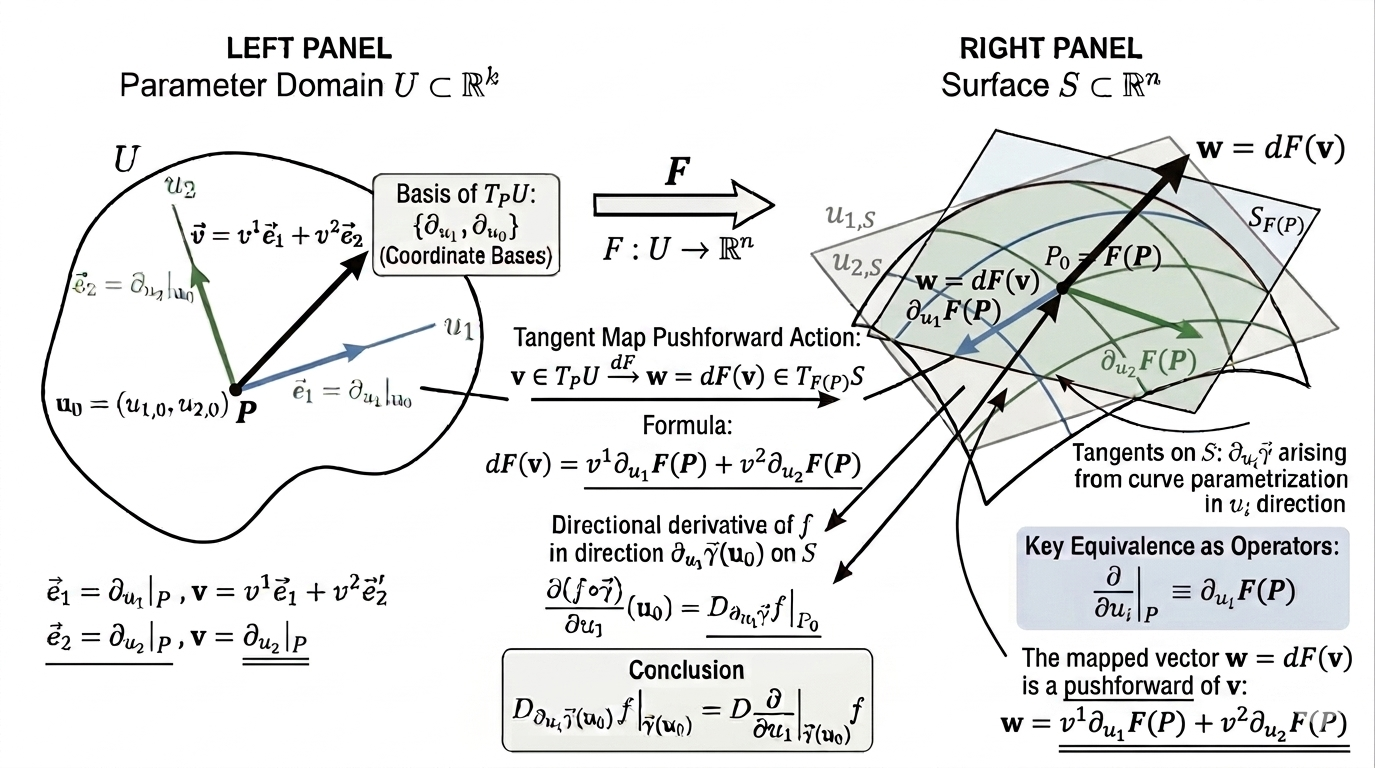
Suppose that \(F: U\subset \bbR^{m}\mapsto \bbR^{n}\) is differentiable, then for any \(P\in U\text{,}\)\(DF(P)\) is a linear map from \(\bbR^{m}_{P} \) to \(\bbR^{n}_{F(P)}\) mapping \(\bv\) to \(DF(P)\bv\text{,}\) and is denoted as \(F_{*}(P)\text{,}\) and is often called the tangent map (or even called the differential and denoted as \(dF\)) of \(F\) at \(P\text{.}\)
namely, to treat \(F_{*}\left(\frac{\partial }{\partial u_{i}}\right)\) as tangent vector \(\partial_{u_i}F(P)\) at \(F(P)\text{.}\) When \(F\) is a parametrization map, we have identified in our notation \(F_{*}\left(\frac{\partial }{\partial u_{i}}\right)\) with \(\left(\frac{\partial }{\partial u_{i}}\right)\text{.}\)
Note that \(F_{*}(P)\) is determined in terms of the first derivatives of \(F\text{,}\) so a more accurate notation would have been \(DF(P)\) or \(dF(P)\text{,}\) but it has been a traditional to use \(DF(P)\) as the matrix representation of \(F_{*}\) under the chosen coordinates.
The geometric interpretation of the linear map \(F_{*}: {\mathbb R}^{m}_{P} \mapsto
{\mathbb R}^{n}_{Q}\) is seen as follows. For any \({\bv}\in {\mathbb R}^{m}_{P}\text{,}\)\(P+t{\bv}\) is a curve in \({\mathbb R}^{m}\) passing through \(P\) with tangent \({\bv}\) at \(t=0\text{,}\) and \({\mathbf x}(t):=F(P+t{\bv})\) is a curve in \({\mathbb R}^{n}\) passing through \(Q\) at \(t=0\text{,}\) its tangent at \(t=0\) is
We note that many books use \(f^{*}\) to denote \((df)^{*}\text{,}\) and \(F^{*}\) to denote \((dF)^{*}\text{.}\) Thus we have the corresponding relation \((f\circ F)^{*}=F^{*}\circ f^{*}\text{,}\) and the pull-back operation behaves like substitution in the differential: \(f^{*}(dz)=df(\bx)
=\sum_{i=1}^{n}\frac{\partial f}{\partial x_{i}} dx_{i}\text{,}\) etc.
Some of these definitions and operational rules may seem abstract and formal. But they are mostly the chain rule in different disguise and capture the essence of differential calculus. In particular, the pull-back operation is essentially the substitution rule for differentials: \(dx_{i}, i=1,\cdots, n\) may be considered as differential forms in \(\bbR^{n}\text{,}\) and when \(x_{i}=F_{i}(\bu)\) is a differentiable function of \(\bu\in \bbR^{m}\text{,}\)\((dF_{i})^{*}(dx_{i})\) is just to substitute \(x_{i}=F_{i}(\bu)\) to get \(dx_{i}=\sum_{j=1}^{m} \frac{\partial F_{i}}{\partial u_{j}}du_{j}\) as a one form in the \(\bu\) space.
Part of the reason for the complication of the notation is that it needs to reflect the dependence on the base point and the tangent vector. For instance, \(\left( dF(\bu)\right)^{*}(\alpha)\) is well defined when \(\alpha \in \bbR^{n*}_{F(\bu)}\) and needs to act on a tangent vector \(\bv \in \bbR^{m}_{\bu}\text{.}\)
Relying entirely on parentheses as delimiters for different inputs and operations can be tiring, so we often use braket notation \(\langle \alpha, \bv \rangle\) to denote \(\alpha (\bv)\text{.}\) In this notation, we have
The pull-back operation \(\left( dF(\bu)\right)^{*}\) has the advantage that for any differential form \(\alpha(\bx)\) defined on \(\bbR^{n}\) (or on a surface in \(\bbR^{n}\)), \(\left( dF(\bu)\right)^{*}(\alpha)\) is a well defined a differential form in the \(\bu\) variable in \(\bbR^{m}\) making it possible for us to do computations in the Euclidean parameter domain, while for a vector field \(V(\bu)\) in the \(\bu\) variable, \(dF(\bu)(V(\bu))\) defines a vector at \(\bbR^{n}_{F(\bu)}\text{,}\) but it may not be considered as a vector field in the \(\bx\) variable, as there may be \(\bu'\ne \bu\) such that \(F(\bu')=F(\bu)\text{,}\) and \(dF(\bu')(V(\bu'))\) may not equal \(dF(\bu)(V(\bu))\text{.}\)
Our consideration for the dual space of the space of tangent vectors and the pull-back maps on tensors is because they provide a natural setting for us to relate \(M\) to \(N\) whenever there is a differentiable map \(F: M\mapsto N\text{.}\) For our specific problem of developing an integration theory on differential forms, we often take \(M\) to be a standard cell (such as a cube or simplex) in \(\bbR^{m}\text{,}\) the pull-back maps allow us to represent forms on \(N\) as forms on the cell in the Euclidean space and use the developed integration theory in the Euclidean space as a tool.
Let \((x, y, z)=F(u, v)=(u^{2}-v^{2}, 2u v, 1)\text{.}\) Compute \(F_{*}(\frac{\partial }{\partial u})\text{,}\)\(F^{*}(y dx + z dy)\) and \(F^{*}(dx\wedge dy + dy\wedge dz)\text{.}\)